 BYD Tech
In short
A vector index finds the vectors closest to a query without comparing the query with every stored vector. Exact search is simple and always right but scales with the size of the collection, so most systems use an approximate nearest neighbor (ANN) index that trades a little recall for much lower latency. HNSW walks a layered graph, IVF scans only the clusters nearest the query, product quantization compresses vectors into short codes, and DiskANN keeps the graph on an SSD; the right one depends on your recall target, memory budget, update pattern and filters.
Key points
- Exact kNN is the baseline and the ground truth: below a few hundred thousand vectors, or for rare queries, it is often fast enough.
- Every ANN index trades recall, latency and memory against each other; measure recall@k against exact search, never assume it.
- HNSW gives high recall at low latency and costs the most memory;
M,efConstructionandefSearchare its knobs. - IVF clusters vectors with k-means and scans only
nprobeof itsnlistlists; it builds fast but must be trained on data that looks like what you store. - Product quantization stores a vector in a few bytes and estimates distances with table lookups; rescore the top candidates with full vectors.
- Filters are where ANN recall quietly breaks: filtering after the search can return fewer than k results.
Exact kNN and why approximate search exists
Semantic search, the retrieval step of RAG and recommendation all reduce to one operation: given a query vector, return the k stored vectors closest to it. The exact way is a linear scan. Compute the distance from the query to every vector, keep the k best. For N vectors of d dimensions that is N times d multiplications per query, it needs no index, and it is always right.
A linear scan is fine for longer than people expect. With normalized vectors the distance is a dot product, which modern CPUs and GPUs compute very fast, and a few hundred thousand vectors scan quickly. The Faiss guidelines suggest exact search when you run only a few searches, because the time to build an index would never pay itself back. Exact search is also the ground truth every approximate index is measured against, so you need it even when you do not serve with it.
import heapq

def dot(a, b):
    return sum(x * y for x, y in zip(a, b))

def knn_exact(query, vectors, k=10):
    # vectors: dict of id -> unit-length vector. Cost: N * d per query.
    return heapq.nlargest(k, vectors, key=lambda i: dot(query, vectors[i]))

def recall_at_k(approx_ids, exact_ids):
    # Share of the true top k that the approximate search returned.
    return len(set(approx_ids) & set(exact_ids)) / len(exact_ids)

vecs = {"a": [0.6, 0.8], "b": [1.0, 0.0], "c": [0.0, 1.0], "d": [0.8, 0.6]}
exact = knn_exact([0.6, 0.8], vecs, k=2)
print(exact)                            # ['a', 'd']
print(recall_at_k(["a", "c"], exact))   # 0.5
At tens of millions of vectors, or at high query rates, the scan becomes the bottleneck, and in high dimensions classic space-partitioning structures such as k-d trees stop pruning much. Approximate nearest neighbor (ANN) indexes give up the guarantee: they inspect a small part of the collection that probably holds the nearest neighbors, and sometimes miss one. For how embeddings and distance measures work, see text embeddings explained.
Recall, latency and memory
Three numbers describe an ANN index, and you cannot maximize all of them at once.
- Recall@k: the share of the true k nearest neighbors, found by exact search, that the index returned. A recall@10 of 0.95 means that on average 9.5 of the true top 10 came back.
- Latency and throughput: time per query, usually read at a high percentile such as p99, and queries per second at a given hardware budget.
- Memory: bytes per vector for the vectors themselves plus the index structure, and whether all of it must sit in RAM.
Every index has a search-time knob that moves along the recall and latency curve: efSearch in HNSW, nprobe in IVF. Turn it up and the index looks at more candidates, so recall rises and latency rises with it. Build-time settings decide which curve you are on, and how much memory it costs. Build time and update behavior matter too: some indexes need a training step on sample data, and some cannot delete a vector cleanly.
Recall of the index is not the same as answer quality. A RAG system that misses the ninth nearest chunk out of ten may lose nothing, while one that misses the single passage holding the answer fails. Measure index recall against exact search, and measure the whole pipeline separately, as in how to evaluate RAG.
HNSW: a layered graph
Hierarchical Navigable Small World graphs (Malkov and Yashunin) are the default index in many vector databases. Each vector is a node linked to a set of near neighbors. Every node is on the bottom layer; when a node is inserted it also gets a random top layer, drawn from a distribution that decays exponentially, so each layer up holds far fewer nodes. The upper layers are a sparse network of long links, like the express lanes of a skip list, and the bottom layer is dense.
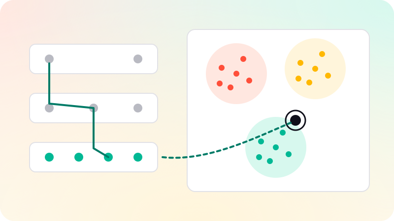
A search starts at a fixed entry point on the top layer and walks greedily toward the query: move to whichever neighbor is closer, until none is. Then it drops a layer and repeats from there. On the bottom layer it runs a best-first search that keeps a list of the ef best candidates found so far and stops when no unexplored candidate can improve that list. The authors credit the layered structure with logarithmic complexity scaling. Inserting a vector is a search for its neighbors followed by linking to them, so the index grows one vector at a time with no training step.
| Parameter | What it controls | Trade-off |
|---|---|---|
M | Links per node on the upper layers; the bottom layer allows twice as many in the paper | Higher gives better recall on high-dimensional data and uses more memory, which grows in proportion to M |
efConstruction | Candidate list size while inserting | Higher builds a better graph and builds more slowly; the paper says it should be large enough for construction recall near 0.95 |
efSearch | Candidate list size at query time, at least k | The main recall and latency dial; can change per query |
The paper calls 5 to 48 a reasonable range for M. As one example of defaults, pgvector uses m = 16, ef_construction = 64 and hnsw.ef_search = 40, and its README advises leaving them alone unless recall is low.
- Memory: the graph links come on top of the vectors. The paper estimates about 60 to 450 bytes of links per object for typical
Mvalues; the Faiss wiki gives roughlyd * 4 + M * 2 * 4bytes per vector for a float32 HNSW index. At 768 dimensions andM= 32 that is about 3,300 bytes per vector, almost all of it the vector itself. - RAM: graph search jumps between random nodes, so HNSW wants the whole index in memory. Paging it from disk makes it slow.
- Deletes: a node cannot simply be removed without breaking paths through it. Faiss does not support removing vectors from its HNSW index; other implementations mark a node as deleted and skip it in results, and many deletes degrade the graph until it is repaired or rebuilt.
- Build: inserting is a search per vector, so building is slower than IVF. pgvector notes that builds are much faster when the graph fits in
maintenance_work_mem.
IVF: clusters and inverted lists
An inverted file index (IVF) partitions the space. A coarse quantizer, usually k-means, is trained on a sample of vectors to find nlist centroids. Each stored vector goes into the list of its nearest centroid. At query time the index finds the nprobe centroids nearest the query and scans only those lists, exactly. With nprobe equal to nlist it is a full scan; with nprobe = 1 it scans one list and misses any neighbor that sits just across a cluster boundary.
import random

def l2(a, b):
    return sum((x - y) ** 2 for x, y in zip(a, b))

def nearest(v, cents):
    return min(range(len(cents)), key=lambda c: l2(v, cents[c]))

def train(vectors, nlist, iters=10):
    cents = random.sample(vectors, nlist)     # coarse quantizer: plain k-means
    for _ in range(iters):
        groups = [[] for _ in cents]
        for v in vectors:
            groups[nearest(v, cents)].append(v)
        cents = [[sum(c) / len(g) for c in zip(*g)] if g else old
                 for g, old in zip(groups, cents)]
    return cents

def build(items, cents):                      # items: (doc_id, vector) pairs
    lists = [[] for _ in cents]               # one inverted list per centroid
    for doc_id, v in items:
        lists[nearest(v, cents)].append((doc_id, v))
    return lists

def search(q, cents, lists, k=10, nprobe=4):
    probe = sorted(range(len(cents)), key=lambda c: l2(q, cents[c]))[:nprobe]
    cands = [it for c in probe for it in lists[c]]   # scan nprobe lists only
    return [d for d, v in sorted(cands, key=lambda it: l2(q, it[1]))[:k]]
Choosing nlist and nprobe has published starting points. The Faiss guidelines suggest between 4 and 16 times the square root of N clusters for collections under a million vectors, trained on 30 to 256 times as many vectors as clusters. pgvector suggests rows divided by 1,000 lists up to a million rows and the square root of the row count above that, with probes starting at the square root of lists; its default ivfflat.probes is 1.
- IVF needs data before it is built. pgvector says to create the index after the table has data; an index trained on too little data returns fewer results than expected.
- The centroids are fixed at training time. If new data drifts away from the training sample, lists grow unevenly and recall drops for the same
nprobe. Retrain and rebuild when the distribution changes. - IVF-Flat stores each vector plus an ID, with no graph links, so it uses less memory than HNSW and builds faster. pgvector's README says HNSW has the better speed and recall trade-off.
- Deletes are easy: remove the entry from its list.
Product quantization and IVF-PQ
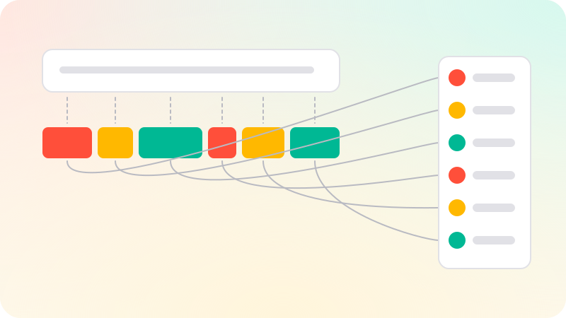
HNSW and plain IVF still store every full vector. Product quantization (Jégou, Douze and Schmid, IEEE TPAMI 2011) compresses them. Split each d-dimensional vector into m subvectors, run k-means separately in each subspace to learn a codebook, usually 256 centroids so each code fits in one byte, and store a vector as the m centroid IDs. A 768-dimension float32 vector takes 3,072 bytes; with m = 96 and 8-bit codes it takes 96 bytes, 32 times smaller. The Faiss wiki gives the code size as ceil(M * nbits / 8) bytes per vector, where M is the number of subquantizers.
Search does not decompress anything. With asymmetric distance computation, the query stays exact: for each of the m subspaces, compute its distance to all 256 centroids once, giving an m by 256 table. The approximate distance to any stored vector is then m table lookups and additions instead of d multiplications.
def l2(a, b):
    return sum((x - y) ** 2 for x, y in zip(a, b))

def split(v, m):
    s = len(v) // m                       # d must be divisible by m
    return [v[j * s:(j + 1) * s] for j in range(m)]

def pq_encode(v, codebooks):
    # codebooks: one list of centroids per subspace, trained with k-means
    return [min(range(len(cb)), key=lambda c: l2(sub, cb[c]))
            for sub, cb in zip(split(v, len(codebooks)), codebooks)]

def adc_table(q, codebooks):
    # Once per query: distance from each query subvector to every centroid
    return [[l2(sub, c) for c in cb]
            for sub, cb in zip(split(q, len(codebooks)), codebooks)]

def adc_distance(code, table):
    # Per stored vector: m lookups and adds, no multiplications
    return sum(table[j][c] for j, c in enumerate(code))
The paper also combines the two ideas in a scheme it calls IVFADC, known in Faiss as IVF-PQ: an inverted file picks the lists to scan, and the vectors in them are stored as PQ codes of their residual, the difference between the vector and its list's centroid. Encoding the residual is more accurate than encoding the raw vector, because residuals are small and the same code bits describe them more precisely. This is how indexes over hundreds of millions of vectors fit in RAM.
- PQ distances are estimates, so top results come out slightly out of order. Fetch more candidates than you need and rescore them with full-precision vectors from disk, the same oversampling pattern used with binary quantization.
- PQ needs training data, like IVF, and the codebooks go stale if the data drifts.
- Variants rotate the space before splitting it (OPQ) so each subspace carries a similar share of the information. The Faiss guidelines recommend OPQ with PQ when memory matters most.
DiskANN and Vamana: indexes that live on SSD
Graph indexes are fast because they live in RAM, and RAM is the expensive part at a billion vectors. DiskANN (Subramanya and colleagues, NeurIPS 2019) moves the graph and the full-precision vectors to an SSD and keeps only PQ-compressed vectors in memory. The compressed vectors steer the walk through the graph; the full vectors, read from disk along the way, give exact distances for the final ranking.
The hard part is reading the SSD as rarely as possible, because every hop of the walk is a random read. The paper's graph, Vamana, is a single-layer graph with a degree bound R and a pruning rule with a parameter alpha. With alpha greater than 1 it keeps some longer edges, so a search reaches the right region in fewer hops. The authors note that HNSW and NSG effectively use alpha = 1, and they aim to cut SSD reads per query to a few dozen.
The authors report indexing a billion points on a single workstation with 64 GB of RAM and an inexpensive SSD, and on the SIFT1B dataset serving over 5,000 queries per second with under 3 ms mean latency at more than 95% 1-recall@1 on 16 cores. Disk-based graph indexes suit very large collections where RAM is the constraint. Below that scale, an in-memory index is simpler.
Filtering with ANN: pre-filtering, post-filtering and in-graph filters
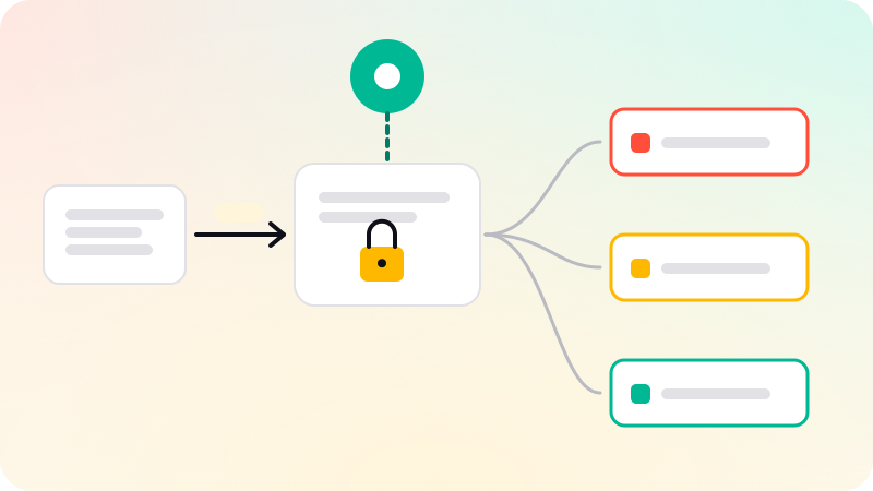
Real queries come with conditions: this tenant only, documents the user may see, published after a date. An ANN index orders vectors by distance and knows nothing about those fields, and how the two are combined decides both recall and latency.
| Strategy | How it works | Where it breaks |
|---|---|---|
| Post-filtering | Run the ANN search for k or a few more candidates, then drop those that fail the filter | A selective filter leaves fewer than k results, sometimes none |
| Pre-filtering with exact search | Find matching IDs with an ordinary index, then scan only those vectors exactly | Exact and simple, but slow when the filter matches a large share of the collection |
| Filtering inside the index | The graph walk skips non-matching nodes but keeps searching until it has k matches | With very selective filters the walk visits most of the graph, or the matching nodes are poorly connected |
| Partitioning | A separate index, partition or partial index per tenant or common filter value | Many small indexes to build and maintain |
The pgvector README gives a concrete example of the post-filtering problem: the index is scanned before the WHERE clause is applied, so with HNSW at the default ef_search of 40 and a condition that matches 10% of rows, a query returns only about 4 rows on average. Its fix is iterative index scans, which keep scanning the index until enough rows pass the filter, with hnsw.iterative_scan and a cap on how many tuples are scanned. It also suggests a B-tree index on the filter column for selective filters, and partial indexes or partitioning by the filter value.
Weaviate's documentation describes the in-index approach: it builds an allow list of matching IDs from an inverted index and the HNSW search considers only those, and when a filter becomes too restrictive it switches to a flat brute-force search over the matches. It also describes ACORN, a traversal strategy it calls especially useful when the filter has low correlation with the query vector. The common lesson: decide which fields you filter on before you build the index, and test recall on filtered queries, not only unfiltered ones. For tenant isolation as a design question, see multi-tenant architecture.
Comparing the index types
| Index | How it searches | Memory per vector | Build and training | Updates and deletes | Good fit |
|---|---|---|---|---|---|
| Flat (exact) | Scans every vector | The vector only | None | Trivial | Small collections, ground truth, very selective filters |
| HNSW | Greedy walk down a layered graph | Vector plus graph links, all in RAM | No training; slower build | Inserts are incremental; deletes are hard | High recall at low latency when RAM allows |
| IVF-Flat | Scans the nprobe nearest clusters | The vector plus an ID | k-means training; fast build | Easy, but drift needs retraining | Large collections, faster builds, less memory |
| IVF-PQ | Scans nearest clusters using compressed codes | A few dozen bytes plus an ID | k-means plus codebooks | As IVF | Very large collections in limited RAM, with rescoring |
| DiskANN | Graph walk guided by in-memory PQ codes, graph on SSD | PQ codes in RAM; graph and vectors on disk | Graph build plus PQ training | Depends on the implementation | Hundreds of millions to billions of vectors |
- Start with exact search if the collection is small. It removes a whole class of recall bugs, and you can add an index later.
- Choose HNSW when the index fits in RAM and you need high recall at low latency, which describes most RAG systems.
- Choose IVF when build time or memory matters more, or when the data is loaded in bulk and rarely deleted.
- Add PQ, or the int8 and binary quantization described in text embeddings explained, when memory is the constraint, and rescore with full vectors.
- Whether the index lives in a dedicated vector database or an extension of the database you already run is a separate decision; see what is a vector database. For how B-tree indexes differ, see database indexing explained.
How to benchmark an ANN index
ANN-Benchmarks (Aumüller, Bernhardsson and Faithfull) is the standard public comparison. It runs many libraries over a sweep of parameter settings on fixed datasets such as sift-128-euclidean and glove-100-angular, with k = 10, and plots recall against queries per second, so each library appears as a curve rather than one number. The paper's headline finding is that very different approaches reach comparable quality and performance trade-offs, which is a reason to test on your own data rather than pick by reputation.
- Take a sample of real queries, or held-out documents used as queries, and the vectors you will actually store, with the real model and dimensions.
- Compute the exact top k for every query with a flat scan. That is the ground truth.
- Build each candidate index and sweep its search knob,
efSearchornprobe, recording recall@k, p50 and p99 latency, and throughput at each setting. - Compare at a fixed point: the recall each index reaches within your latency budget, or the latency each needs to reach your recall target. A single average hides the trade-off.
- Record memory, build time and index size, and repeat the measurement with your real filters and with inserts and deletes running.
- Re-run the benchmark when the data, the embedding model or the index settings change.
Measure with warm memory and with the concurrency you expect, and report percentiles rather than means. Then measure end-to-end retrieval quality, because the ranking that reaches the user often passes through hybrid search and a reranker after the index.
If you want vector search or a RAG feature built into your product, see our AI agent development service: the code lives in your GitHub from day one, and AI-assisted work is reviewed by an engineer.
Sources
Checked when this post was written.
- Malkov and Yashunin, Efficient and robust approximate nearest neighbor search using Hierarchical Navigable Small World graphs (arXiv)
- Jégou, Douze and Schmid, Product Quantization for Nearest Neighbor Search (IEEE TPAMI, 2011)
- Subramanya et al., DiskANN: Fast Accurate Billion-point Nearest Neighbor Search on a Single Node (NeurIPS 2019)
- Douze et al., The Faiss library (arXiv)
- Faiss wiki: Guidelines to choose an index
- Faiss wiki: Faiss indexes
- Aumüller, Bernhardsson and Faithfull, ANN-Benchmarks: A Benchmarking Tool for Approximate Nearest Neighbor Algorithms (arXiv)
- ANN-Benchmarks results
- pgvector README (GitHub)
- Weaviate documentation: Filtering